本文共 1849 字,大约阅读时间需要 6 分钟。
机械革命Z3 Pro使用的是一块可自定义RGB的紧凑型全尺寸背光键盘,按键采用侧边全透光设计,让玩家即使在黑暗的环境下也能轻松掌控操作。选机械革命z3pro还是x8pro这些点很重要看过你就懂了
机身A/C面采用的是航空喷砂铝镁合金材质,并且整机将重量压缩到了2KG以内,机身厚为23.6mm,集轻薄与高性能于一身。作为一台游戏本,散热是决定硬件性能释放的重要因素。机械革命Z3 Pro搭载全新升级的第六代智能散热系统,采用底部镂空加后、侧面多出风口的散热设计,对比上代产品风量提升35%。
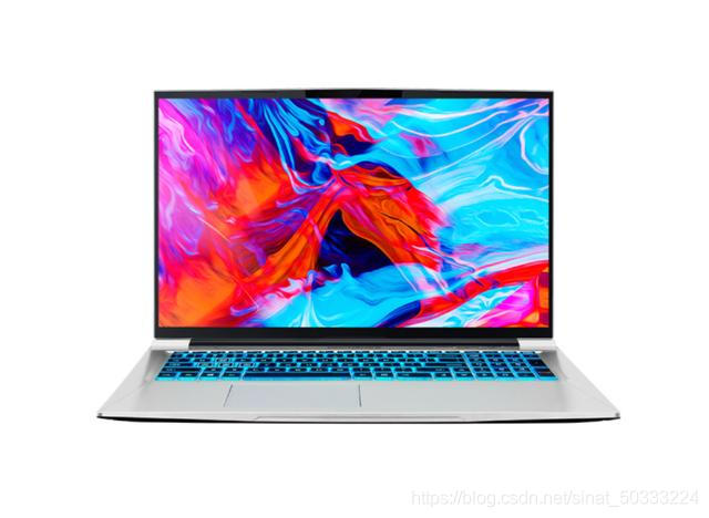
机械革命Z3 PRO机型搭载的是GeForce RTX 3060 Laptop GPU,配备一块15.6英寸240Hz的高刷新率电竞屏,并且拥有100%sRGB色域。标配16GB DDR4内存,i7-10875H处理器,基本能够保证GeForce RTX 3060 Laptop GPU的性能释放,不会因为其他硬件性能造成瓶颈问题。
机械革命Z3 pro游戏本包装保护:包装很严实,不用怕损坏。外形外观:外观虽然说是游戏本,但是比较低调。在正式场合也不会显得突兀。画面品质:画质很清晰,稳妥。运行速度:感觉挺快的游戏效果:打游戏完全不卡就对了包装保护:包装简单环保,无破损外形外观:做工细致,大气简约,比预想的厚一些画面品质:画质细腻,效果好评测评测:开高特效无卡顿,非常流畅运行速度:飞一般的感觉游戏效果:综合各方面达到游戏本的最高水平机械革命z3pro和x8pro包装保护:包装简单简洁,保护得很好。外形外观:暗黑色有上档次,炫红色灯光的键盘很好看。机器很薄,屏幕也很薄。画面品质:很清晰,画质很好。运行速度:挺好,内存大,很顺畅。游戏效果:不卡顿,满意。包装保护:包装很严实,收到货无缺脚,很放心外形外观:外观采用背光大灯设计,用起来倍有面子,尽显奢华画面品质:采用144hz的屏幕,跟2060卡对应,比60hz的画面体验好了不止一点评测评测:评测很高运行速度:速度特别快,玩游戏办公完全不是问题游戏效果:玩吃鸡之类游戏没问题
机械革命Z3 pro游戏本站神系列,对于一个刚上大学的孩子来说,性价比因该是最高的,男孩玩玩游戏,同等价位,配置相当不错,一般的大型游戏跑起来都很流畅,都说事故率高,目前还没发现,用了快一个月,各方面都很流畅,散热也还好,噪音能接受,屏幕分辨率也能满足要求商家快递的物流真的很快 第一天付完款 第二天的下午就收到货了 好评 支持国产包装保护:包装完好,没有损坏。外形外观:外观A面有灯,接口多,键盘带走小键盘且回弹舒适。画面品质:高色域画质不论看电视还是游戏都很舒适,对比之前的笔记本,画质根本不是一个级别。评测评测:新电脑开机评测24万多,如果内存大还可以评测更多。运行速度:速度很快,不管干嘛都不影响!游戏效果:游戏体验奈斯,有散热模式切换,体验更完美!
机械革命z3pro和x8pro邮递很快,一天就到家了。一直用戴尔的牌子,新出的G5真的别具创新!外观是布灵布灵的反光材质,渐变色的logo,加上键盘背光灯,和一条灯带,外星人灯光特效加持,游戏真的爽!十代i7加上RTX2060显卡,游戏办公两不误,性价比超高。朋友看我买的这款机器不错,也让我帮忙买,买了N台了吧。这款电脑绝对是入门的旗舰产品,一起玩游戏联网组队真的太棒了,声音悦耳清新,音效效果极佳;内置外星人控制中心,管理你的游戏等等非常实用的;还要说就是屏幕的色彩真是太赞了,色彩饱和度非常高,尤其是在日光灯下,比45%的好的不知道多少,对对手的识别和发现简直快好多,被KO的风险大大降低,还有比这更重要的吗
机械革命Z3 pro游戏本用于设计专业的小宝宝们 这个款机器帮你解决所有的问题了哦 高色域,喜欢的可以尽快入手啦 哈哈 好不容易买的宝贝呢 机器拿回来时候检测了一下 鲁大师评测超给力呢 很赞 这个屏幕和其他的机器很不一样 是属于有点防眩光屏的感觉 看着非常高大上 一直都很喜欢戴尔的这个品牌 因为质量非常好 品牌也很给力 优惠力度大 喜欢的宝宝们可以尽快入手了 因为效果很赞呢 有好多其他的版本哦 可以不同的升级 因为我是用于作图所以我买的这个完全够用 嘻嘻 还会一直支持戴尔的这个品牌的首发价格优惠,还很抢手,等了几天终于到货了,电脑包装保护安全严实,外形外观大气,同配置对比性价比高,15.6英寸显示屏,1080P分辨率,72%NTSC色域,144Hz高新率,还没开始使用,期待使用体验。
转载地址:http://wxfaz.baihongyu.com/